Introduction

The collection frequency structure describes whether the collection frequency remains the same throughout the year, changes seasonally according to a fixed pattern, or can be selected by residents. In Germany, seasonally changing collection is mainly applied during periods of high vegetation growth, when larger quantities of biowaste arise. More frequent collection may also be required during summer because food waste degrades faster and generates odours. Under a flexible structure, residents can usually select a collection frequency at the beginning of the year, which may also affect the cost of the waste collection service.

The collection count describes the number of scheduled collections per year for a specific waste stream.

The collection count ratio allows a direct comparison between two waste streams, in this case biowaste and residual waste. It is calculated by dividing the annual collection count for biowaste by that for residual waste. For example, a ratio of 1 indicates that both waste streams are collected equally often.

 

Descriptive overview

Influencing factor overview

Two collection frequency structures are used in areas with biowaste door-to-door collection. A fixed structure covers 66% of the population (18 collection areas), while a seasonally changing structure covers 34% (12 areas). For residual waste, 89% of the population (28 areas) is covered by a fixed structure and 11% by a flexible structure.

The collection count varies across the collection areas and was clustered into logical sections. For biowaste, 26 collections per year, corresponding to collection every two weeks, apply to 60% of the population (17 areas). A seasonally varying count of 27 – 51 annual applies to 34% (12 areas), while 52 annual collections, corresponding to weekly collection, apply to 6% (1 area). For residual waste, 26 collections per year apply to 68% of the population (21 areas), 13 collections per year, corresponding to one every four weeks, to 27% (10 areas) and 18 collections per year to 5% (1 area).

The calculation of the collection count ratio between both waste streams shows that the same number of collections applies to 30% of the population (8 areas). Biowaste is collected more than once but less than twice as often as residual waste for 24% (10 areas). A ratio of two biowaste collections per residual waste collection applies to 37% (11 areas), while a ratio above two applies to 9% (2 areas).

Spatial distribution

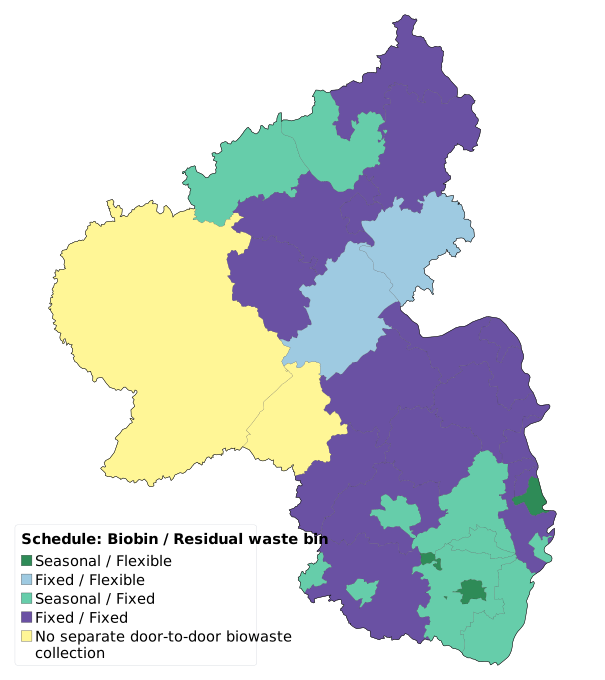
The frequency structure mainly differs in regional clusters, with the dominant combinations occurring in southern and northern parts (seasonally changing and fixed frequencies) and in central and northern parts (both fixed frequencies).

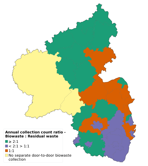
The collection count ratio follows a rather diverse distribution across the region with collections of biowaste twice or more often compared to residual waste occur in a stretch from central south to central north of RLP. Seasonally varying biowaste collection is mainly applied in the southern part of RLP.

Statistical Assessment

The biowaste stream separation rate (SR_BW,gross), the approximated net biowaste separation rate (SR_{BW,approx-net}) and total food waste in residual waste (FW_RW) as mass base were used as key performance indicator (KPI) for the statistical assessment. Figures showing the influence of the assessed influencing factors on biowaste and residual waste quantities are provided in the appendix (Download Factsheet PDF).

The boxplots in Figure 3 indicate differences in SR_BW,gross for the different ratios.

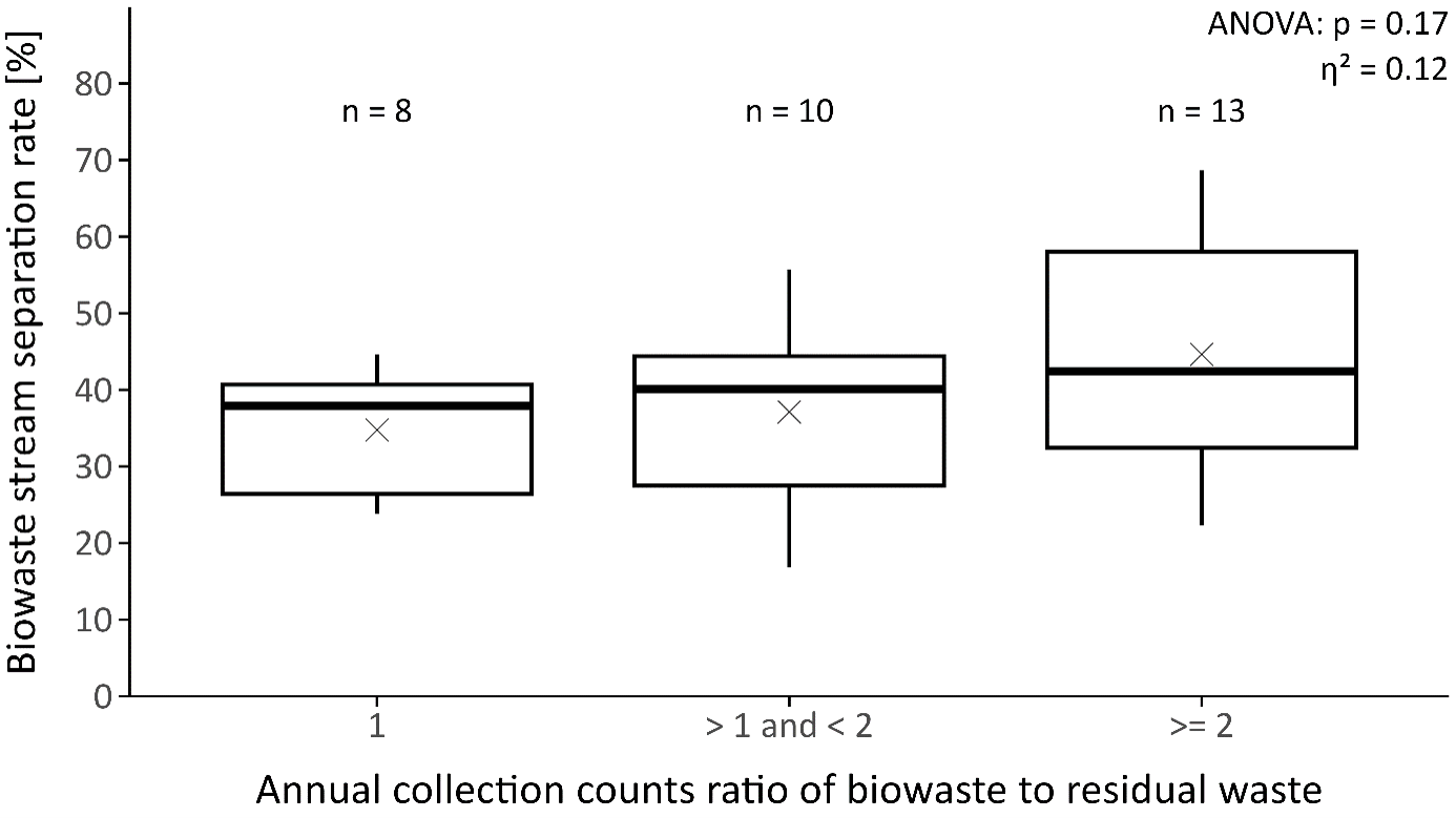
Higher annual collection count ratios of biowaste to residual waste are associated with a gradual increase in SR_BW,gross. Areas with the same number of collections for both waste streams show the lowest median SR_BW,gross of 38% (Q1 = 26%; Q3 = 41%). Where biowaste is collected more than once but less than twice as often, the median increases slightly to 40% (Q1 = 28%; Q3 = 44%). Ratios of two or more show the highest values overall, with a median of 42% and a clearly higher upper quartile (Q1 = 33%; Q3 = 58%). However, the distributions overlap substantially, and variability increases with the collection count ratio.

To allow for a direct comparison with the following SR_{BW,approx-net} (Figure 4), SR_BW,gross was as well analysed with the same sample population. The resulting boxplots can be found in Figure 10 in the appendix.

The boxplots in Figure 4 indicate differences in SR_{BW,approx-net} for the different ratios.

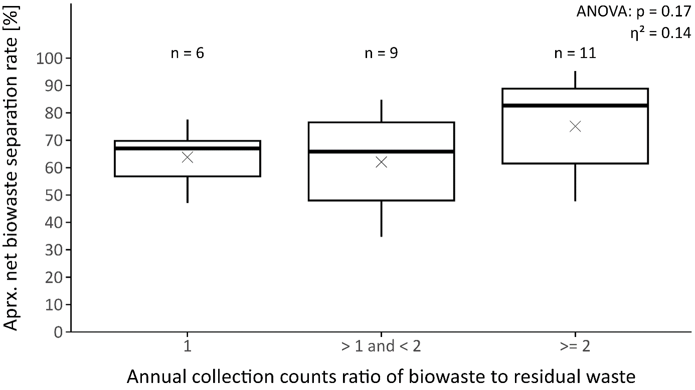
SR_{BW,approx-net} shows a clearer increase at higher collection count ratios compared to SR_BW,gross (The correlation between both KPIs is evaluated in a special Fact Sheet: Link). Areas with the same number of collections for both waste streams have a median of 67% (Q1 = 57%; Q3 = 70%), while ratios above one but below two show a similar median of 66%, but with greater variability (Q1 = 48%; Q3 = 77%). Ratios of two or more show the highest values overall, with a median of 83% (Q1 = 62%; Q3 = 89%). Compared with the gross biowaste stream separation rate, where the median increases only gradually from 38% to 42%, the approximated net rate shows a much stronger difference for ratios of two or more.

The boxplots in Figure 5 indicate differences in FW_RW for the different ratios.

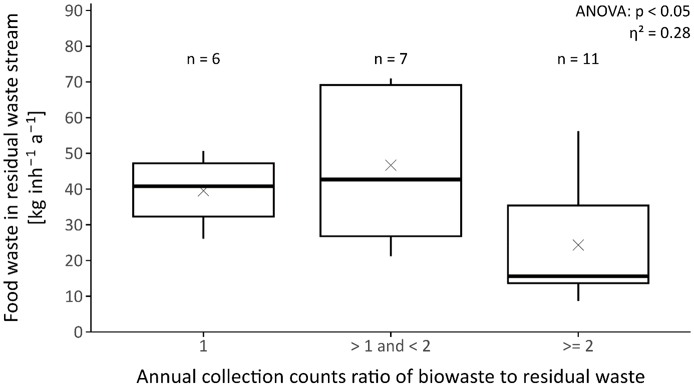
Food waste quantities in residual waste are lowest at higher collection count ratios. Areas with the same number of collections for both waste streams show a median of 41 kg per inhabitant and year (Q1 = 32 kg; Q3 = 47 kg). Ratios above one but below two show a similar median of 43 kg, but considerably greater variability (Q1 = 27 kg; Q3 = 69 kg). Ratios of two or more show clearly lower values overall, with a median of 16 kg per inhabitant and year (Q1 = 14 kg; Q3 = 35 kg). Although the distributions overlap, the overall pattern indicates substantially lower food waste quantities in residual waste where biowaste is collected at least twice as often as residual waste.

Significance testing

For the SR_BW,gross, the one-way ANOVA found no statistically significant differences between the collection count ratio categories (p = 0.165). The same applies to SR_{BW,approx-net} (p = 0.173). Pairwise comparisons also showed no significant differences between the individual categories for either KPI.

FW_RW differed significantly between the collection count ratio categories (ANOVA, p < 0.05). The descriptive results indicate that this difference is mainly related to the lower quantities observed where biowaste is collected at least twice as often as residual waste. However, none of the pairwise comparisons remained statistically significant after adjustment for multiple testing.

Effect size

For SR_BW,gross, the effect size was η² = 0.12. This indicates that around 12% of the observed variation can be associated with the collection count ratio, corresponding to a medium-to-large effect. The effect was slightly stronger for SR_{BW,approx-net} (η² = 0.14), representing a large effect.

The largest effect was found for FW_RW (η² = 0.28). The result indicates a large effect and supports the descriptive pattern of considerably lower food waste quantities where biowaste collection occurs at least twice as often as residual waste collection.

 

Conclusion

Across all three KPIs, the results show a consistent overall trend: biowaste separation performance improves as biowaste is collected more frequently than residual waste. Both separation-rate indicators reach their highest values at collection count ratios of two or more, while food waste quantities in residual waste are clearly lowest in this category. The effect sizes indicate that the collection count ratio is an important influencing factor in practical terms, even though the data of the different categories partly overlap.

The clearest pattern is found for FW_RW. The more frequently biowaste is collected in relation to residual waste, the less food waste remains in the residual waste stream. The available data do not show whether this results from better separate collection or greater food waste prevention, as no composition data were available for the separately collected biowaste. However, the parallel increase in SR_BW,gross and SR_{BW.approx-net} suggests that improved separate collection is likely to be an important explanation.

The results therefore support aiming for biowaste collection at least twice as often as residual waste. This provides more regular disposal opportunities for biowaste, particularly food waste, and reduces the incentive to use the residual waste bin for it. Where both streams are collected equally often, the timing of collection may also matter. If biowaste and residual waste are both collected every two weeks on alternating weeks, residents may be encouraged to place food waste in the residual waste bin the week before its collection.

 

Downloads

Fact Sheet PDFCase Study Profile PDF